I Introduction
II
Spatial & Temporal Coverage
III Procedure
Details:
We compute upwelling and downwelling fluxes and cloud forcings, at the surface and top of atmosphere, for each of 516 grid locations at each pole, every 3 hours. The International Satellite Cloud Climatology Project (ISCCP) D1 data set provides cloud, atmospheric, and surface information at 3 hour intervals. The atmospheric profile information is supplemented by the TOVS Pathfinder PathP data sets when available (and they are only available for the Arctic). A neural net (a specialized version of Fluxnet) has been trained to compute the fluxes with the results from Streamer computations on a small subset of the full 9 years of data.
The PRFI procedure compiles the necessary inputs to the neural net from the ISCCP D1 and the Pathfinder PathP data sets, feeds the inputs to the net, and writes the resulting fluxes to an output file (one file per day). To produce more focused neural nets, we have chosen to use two Fluxnet implementations, one for cloudy cases, one for clear.
The inputs to each net are listed below:
(38 35 TOTAL NUMBER OF INPUTS)
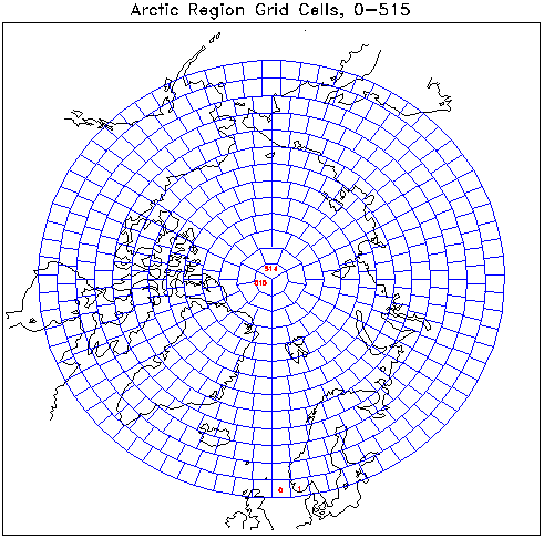
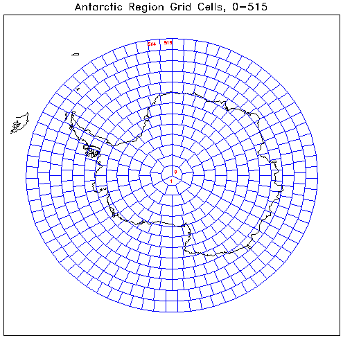
The fluxes are generated every 3 hours for 516 grid cells in each polar region, extending down to 57.5° latitude. The grid structure is an equal area mapping, with cell size defined by the area of a 2.5° × 2.5° region at the equator, giving an equivalent square cell of side 280 km. This is the grid system used by the ISCCP; see their DX/D1/D2 data set documentation for details. The figures below show the cell grids for each pole. Since it is not a square array grid, the output is not formatted as a square array (image) structure; rather, geographic coordinates of each of the 516 locations are provided in a separate array. Note the cell numbers increase in a counter-clockwise spiral towards the pole for the Arctic, and in a clockwise spiral away from the pole in the Antarctic. To download a UNIX compressed (".gz"), postscript file containing grid cell maps with complete numbering please click here.
Temporally, the ISCCP data set provides data at 3-hour intervals. However, for any given 3-hour period, a significant portion of each polar region has no reported data (presumably due to satellite coverage limitations). A simple data filling scheme was defined to deal with the missing data. Please see the Data Filling section of this document for further details. Thus, the 3-hourly data set does not contain spatially comprehensive coverages at each 3-hour period. Except for the very occasional occurrence of a cell with no reported data for the entire day, the provided daily averages are spatially complete as are the monthly averages for the entire 9 years of data.
As ISCCP reports different data for day and night, we also have different procedures for flux computations at day and at night, as described below. It is important to note here that ISCCP reports a cell as 'night' when the majority of pixels in that cell have solar zenith angles >= 78.5°, not 90° as one might expect. The same versions of fluxnet (cloudy/not cloudy) are used day or night, only the processing of the data before being sent to fluxnet differs.
The code proceeds by processing separately each cloud type in a cell, plus a clear sky component if present. These separate output fluxes are then weighted by the cell fraction of each cloud type (or clear portion), and summed for the cell, producing the final output fluxes.
To compile the Fluxnet input data, various assumptions and decisions must be made to ensure the input data set represents both physically real cloud, surface, and atmospheric conditions, and conditions within the range of the training data. The primary such assumptions and decisions that were necessary are described below, along with some of the finer details on the compilation of the various input data parameters from the ISCCP and PathP data sets. Refer to the ISCCP D1 data set documentation or variable list for more details on the input variables described below.
ISCCP reports both a clear sky surface temperature (ISCCP D1 item 159), and a composite (#158). We use the clear sky surface temperature when available, and the composite when the clear is not reported.
If the reported surface temperature is above 307 K for cloudy cells,
or 305.8 for clear cells, it is reset to these maxima, which were the highest
surface temperatures found in the training data. Also, if the difference
between the composite and clear sky temperatures is more than 20 K, the
composite temperature is used. This served to eliminate the occurrence
of very high surface temperatures (up to 337K = 64C = 147F), which seemed
clearly unphysical spurious values.
ISCCP reports two albedos: "mean rs from clear sky composite" (item #163) and "mean rs for clear pixels" (item #164). If the latter is available, it is used; if not, the composite measure is used. At night, a value of 0.5 is used, although this has minimal impact on longwave fluxes from Fluxnet.
Very occasionally, unexplained error codes of -200 or -100 are reported in place of either or both ISCCP albedo values, with the rest of the ISCCP data reported as usual. In such cases, an approximate albedo is calculated from surface type information. Generally, the surface type is calculated from the albedo and other considerations (see SURFACE FRACTIONS below); however, in this case, as at night, surface types are calculated from rough information provided by ISCCP (item #6). We then simply turn this around to calculate some approximate albedo, given by:
The solar zenith angles reported in the ISCCP data set are not
the values used in computing fluxes. In order to obtain proper daily
average fluxes, values of the cosine solar zenith angle are calculated
at 30 minute intervals and averaged over the 3 hour interval centered on
the nominal times reported in the ISCCP data. The angle is calculated
from the given coordinates of the center of the ISCCP cell. Calculated
solar zenith angles greater than 100 are set to 100 before being feed to
Fluxnet
- this is the largest value with which Fluxnet was trained.
This is not provided by ISCCP; it is set to 0.1 for Arctic cases, 0.06 for Antarctic.
The neural net was only trained with these two values; however, if other
or variable estimates became available, it would be relatively straightforward
to include variation here and retrain the neural net.
ISCCP reports an ozone level in dobson units. We convert this value
to g/m2 for Fluxnet (multiply by 0.021416669).
In order to compute fluxes, Streamer, which provides the training data for the neural net, requires a surface type. Unfortunately, we are not provided with very good surface type data from either the ISCCP or the PathP data sets. ISCCP provides a surface albedo, a percentage of snow/ice cover (item #7), and a rough code (item #6) indicating that the surface is either (1) 0-35% land, (2) 35-65% land, or (3) 65-100% land (termed 'water', 'coast', 'land', respectively). We have chosen to use the Streamer surface types of open seawater (1), snow (3), and vegetation (5). To calculate the fraction of each type in each cell then requires some assumptions. In the daytime, we determine a best guess of surface type from albedo considerations; at night, rougher estimates are computed from the surface type code.
Daytime:
We determine surface type fractions by maintaining the overall reported albedo and adjusting surface fractions to fit this albedo with fixed visible albedos for the surface types (0.09 for vegetation, 0.12 for water, and 0.83 for snow_ice). Eg:
Nighttime:
At night, lacking albedo information, we simply use the ISCCP surface codes to determine rough surface type fractions. First, we set the snow_ice fraction to the reported snow_ice fraction, and then set either the land or water fraction to (1 - snow_ice), or equally partition the 'coast' type into land and water in that case.
(This was initially also done for daytime determinations; however, due
to problems arising from unrealistically high (higher than Streamer's
built-in values) surface albedos for reported water or land surface types,
we decided to calculate surface type fractions from set albedos as above.)
There are in general two atmospheric temperature profiles available: a 10-level profile included in the ISCCP data set, and a 39-level profile available from the separate TOVS Pathfinder PathP data set (only for the Arctic). The PathP profile is preferred, and used whenever possible; however, at times the ISCCP profile is preferred -- when the PathP is not reported for the cell or day of interest, or when the reported cloud top temperatures correspond to more realistic cloud top pressures with the ISCCP rather than the PathP profile. Generally, if all the cloud top temperatures fall within the temperature range of the PathP profile, that profile is used. If not, then either the ISCCP or the PathP profile may be used - whichever produces fewer errors. Such errors include clouds which do not fit in the physical space between its calculated top height and the surface, given set extinction ratios (31.4 for water clouds, 5.9 for ice). Whichever profile chosen is interpolated to the 21-level profile used to train the neural net.
The PathP profiles are on a different grid than the ISCCP - a 67x67
square grid over the arctic (4489 cells) region covers our 516 cell output
grid (the ISCCP grid, whose cells are nominally 280 km on a side; PathP
are 100 km on a side). The code selects the PathP cell closest
to the center of the ISCCP cell. If the closest cell is not reporting data
for that day, the next closest PathP cell data is examined, etc.
If no PathP cells are found to have good data, within the boundaries of
the ISCCP cell, the ISCCP profile is then used.
Special Case - Above Elevated Land:
If the surface is at some altitude and thus has a surface pressure less than 1000 mb, the profile data will have NODATA values for the levels that fall below the surface. For example, if the surface is at 900mb, then the lowest two temperatures in the 39-level PathP profile will likely be missing (reported as -1000), because they are centered at 927 and 984 mb, higher than the 900 mb surface pressure. However, we need to send a constant number of input units to Fluxnet, irregardless of the surface pressure. To achieve this, we use what are called sigma pressure units. This essentially stretches the reported pressures to the 21 required levels, biased by the reported surface pressure. (The surface pressure is given in the ISCCP data set, item #184.)
The sigma pressure conversion interpolates the given temperature profile
to new 'sigma' pressure coordinates, which are determined from the ratio
of the reported surface pressure to the standard 1000 mb pressure.
Eg (new level)/(surface pressure) = (standard level)/1000 mb.
In other words, we are expanding the reported pressures, from 0 mb to surface pressure, into the 0 to 1000 mb range. Thus, if the surface is at 900 mb, then we multiply the wanted standard level's pressure by 0.9 (giving us sigma coordinates), and interpolate the reported values at the reported pressures to these new coordinates.
Note: ISCCP uses sea level pressure of 1000 mb while PathP uses 1013
mb; currently, this is not adjusted for either way.
The PathP and ISCCP data sets report precipitable water column amounts, for five specified atmospheric layers. We prefer to use the precipitable water (PW) amounts from the same data set (PathP or ISCCP) which we are using for the temperature profile. However, at times, one data set or the other may not report the PW amounts while reporting temperature profiles. In such cases, the code searches for the nearest valid precip water data: first it checks the ISCCP data for the cell of interest, then searches through the PathP cells within the ISCCP cell, and finally searches in an expanding radius outside the ISCCP cell of interest, checking both data sets for valid data. Note that while ISCCP always reports a temperature profile (for any cell for which they are reporting cloud data), they do not always report precip water data.
A 'valid' PW profile contains at least 3 reported values (of the 5 possible, thus allowing for elevated surfaces up to 500 mb), whose total is greater than 0. Occasionally, zero is reported in all levels of a profile (as opposed to the -1000 no-data values), which is clearly not physical; in such cases, the next closest good profile is substituted.
Fluxnet requires water vapor mixing ratios, in g/kg, at five specified levels. To convert from precipitable water layer totals to mixing ratios at layer centers, we use the following relation:
The center pressures of the levels for the PathP precipitable water
amounts are at: [350,450,600,775,925] mb. These same pressure levels
were used for the training of Fluxnet so that the values could be
passed in directly (after conversion from layer amounts) from the PathP
data set. However, ISCCP reports values at: [900,740,620,500,375]
mb, so the calculated mixing ratio values at the ISCCP levels (when using
the ISCCP profile) are interpolated to the pressures of the PathP profiles.
Since the PathP levels cover a wider range, interpolation can lead to negative
values at the ends (for the 350 and 925 levels). Such results are
set to a minimum mixing ratio value (0.005). Also, any interpolations
(or filling in of zero values) are not allowed to exceed a maximum value
of 11.8.
Special Case - Above Elevated Land:
If over an elevated surface, sigma pressure coordinates are used to
scale the pressure levels accordingly, with the layer thickness of the
lowest layer appropriately reduced before its mixing ratio is calculated.
However, this requires an accurate value of the surface pressure to correctly
calculate the mixing ratio. For example, the lowest PathP water vapor
layer extends from 850 to 1000 mb. If the surface is actually at 900 mb,
then the reported precipitable water content actually occupies only 50mb
of atmospheric thickness, not 150 mb. Using a thickness of 50 mb then produces
a much higher mixing ratio than if one ignored the surface pressure correction
and used a thickness of 150 mb. Potential errors may occur if the
surface pressure used for the adjustment is significantly different from
the actual average surface pressure over the cell of interest. Therefor,
because the ISCCP and PathP cells have quite different footprints, it is
possible that the surface pressures provided for the ISCCP cells may not
be the appropriate pressures to use for the much smaller PathP cell, especially
in mountainous regions. Lacking other data sets and with no surface
pressure information included in the PathP data set, we have no better
alternative at this time. Note that when precip water data must be
taken from a nearby cell (either PathP or ISCCP) from the cell of interest
due to missing values, the surface pressure is taken from the closest ISCCP
cell to this location, not simply from the cell of interest. Also,
although this procedure may produce an unrealistically high mixing ratio
in the lowest layer if the surface pressure is not accurate or the layer
is simply very thin, the total column precip water will be maintained.
The ISCCP data reports the amounts (percentage coverage of a cell) and parameters (cloud top temperature and optical depth) of up to 15 different cloud types (6 mid and low level water clouds, 6 mid and low level ice clouds, plus 3 high ice cloud types). PRFI runs each reported cloud type through Fluxnet, and then averages (weighted by the fraction of that cloud type) the resulting fluxes, plus any clear sky, for the cell.
Average values were chosen for water and ice cloud particle radii and water content:
ISCCP reports an optical depth for each reported cloud type present in a cell. However, at night (or polar winter), there is no reported optical depth, but Fluxnet does require this information. To provide a best-guess, we have constructed a data set of average daily optical depths, from daytime optical depth information. Lacking information on nighttime cloud cover patterns, we calculated polar average cloud optical depths for each day, for each pole, and for the reported clouds on that day (e.g.., clear sky was not averaged into the optical depth - this is an average cloud optical depth, not an average sky optical depth). Then, this time-series of daytime averages was interpolated across the winter period (Nov-Feb for the arctic, May-Aug for the antarctic) when there are no daytime clouds to average. When consecutive years were not available in the arctic (eg 1985), the interpolation was done with just that year's fall and winter data (eg Dec 1986 to Jan 1986); since these are simply broad arctic-wide trends, this should not have a significant impact. To provide a little more detail, this procedure was done for three atmospheric levels: 30-440 mb, 440-680 mb, and 680-1000 mb. (ISCCP does report cloud top temperatures for nighttime clouds, so the appropriate level can be determined.) Thus, there are three optical depth values per day, one per level.
At rare times (0 to 15 times per month, usually 20 to 30 times total
per year), ISCCP reports a cloud optical depth of -200 (as opposed to its
traditional -1000 no-data value) for a specific cloud, while reporting
the cloud's other parameters. In such cases, the cloud is simply ignored
and not used in computations (as opposed to inserting some average optical
depth).
Extra Nighttime Cloud Amounts:
The ISCCP reporting of cloud data at night is much less comprehensive than their daytime data, due to a lack of visible information. For our purposes, a significant limitation is in their reporting of cloud top pressure distributions (items #23-29), which is the only vertically stratified reporting of cloud amounts at night. This information is derived solely from IR cloud threshold determinations (what they term "IR-cloudy"), and does not include any near infrared determinations (NI), or, obviously, visible information. Thus, there is a potential discontinuity between daytime cloud amounts and nighttime amounts, with daytime amounts in general higher due to inclusion of visible and NI information.
At night, however, there are some additional cloud amounts, beyond what is given by the IR, reported in their cell-wide total cloud amounts (items 12-19). We have added these to the IR amounts to help reduce any day/night discontinuity. ISCCP data set item #12 reports total cloud amount; item #13 reports IR-cloud; and item #16 reports NI-only cloud amount. Note these are not stratified amounts, just cell totals.
At nighttime, the IR-cloud amount equals the sum of the stratified amounts
(items 23-29), but the total amount is often higher. In general, the total
amount equals the sum of the IR-cloud and the NI-only amounts; however,
in some cases, other adjustments have been made, slightly increasing the
total cloud amount (see ISCCP D1 data set documentation). ISCCP also
reports the cloud top temperature and pressure for the NI-only amount.
Thus, we have added this extra amount (total - IR_cloudy, or item 12 -
item 13) for nighttime cells, in the appropriate layer (depending on cloud
top pressure reported in item 81 for NI-only-cloudy pixels).
The PRFI procedure contains subroutines to return the cloud top pressure and cloud phase for the reported cloud top temperatures of each cloud type, using the atmospheric profile information given by either the PathP or ISCCP data set. First, the PathP profile is used, if available, and all reported cloud types for a given cell and time are evaluated at once by the subroutine. Then, if the routine cannot find an acceptable cloud top pressure for the given temperature for one or more of the clouds, the ISCCP profile is checked to see if it gives better results. Specifically, the ISCCP profile is checked if the any of the following errors are found for any cloud while using the PathP profile:
If the best such cloud parameter determination still produces clouds that are too thick for the given physical space, the cloud optical depth is reduced to what would fit in the physical space between the cloud top pressure and 0.5 km above the surface.
Below are details on the pressure and phase determinations:
Pressure:
If all the temperatures fall within the range of the PathP profile, then the PathP profile will be initially used to determine cloud top temperatures. If they do NOT fall within the PathP range, but do fall within the range of the ISCCP reported profile, then the ISCCP profile will be used. If they do not fall within the ISCCP range either, then the PathP will be used, since it is generally assumed to be a better profile. The code takes care of (eg, ignores) outlier values. If a PathP profile is not available, the ISCCP profile is used.
Occasionally, the ISCCP reports a cloud top temperature (TC, items 113-146) which is BELOW any temperatures reported in the PathP atmospheric profile. In such cases, the cloud top pressure is set to the tropopause pressure (or to 300 mb if there is no reported tropopause pressure). Also, occasionally, a cloud top temperature is reported higher than any PathP profile temperature. In this case, the ISCCP profile is then used. Generally, the ISCCP profile will encompass its own reported cloud top temperatures, so this tends to work. When it doesn't, the pressure is set to the pressure of the highest temp level in the atmosphere, and at least 50 mb above the surface. In any and all cases, cloud top pressures are not allowed any higher (lower in altitude) than surface pressure - 50 mb. If the chosen profile (chosen due to least number of such errors) still indicates a cloud within 50 mb of the surface pressure, that cloud's top pressure is reset to 50 mb above the surface.
Inversions:
A somewhat complicated algorithm was developed to deal with locating cloud top pressures when the temperature profile may have inversions in it. In practice, although inversions are quite common, it is not common for a cloud to be present in the inverted portion of the profile (from what we can determine with the given data). Thus, the following procedure should not be greatly affected the fluxes in general.
To find the pressure corresponding to the reported cloud top temperatures, a continuous, singular profile is required. Unfortunately, inversions in the atmospheric profile allow multiple pressure levels to be at the same temperature, complicating the interpolation. To get around this, the code checks for inversions in the profile. High inversions, near the TOA, are ignored. Low inversions, at the surface, may be used if the cloud is determined to be of low altitude.
This altitude determination is estimated by the numbers of pixels reported in the ISCCP data set for different layers. There are two low layers that are of interest - one extends from the surface to 800 mb ('low'), the other from 800 mb to 680 mb ('high'). Thus, if the number of pixels, for a given cloud, reported in the 'low' layer is higher than the number reported in the 'high' layer, then the cloud is said to be in the low layer.
One catch here: for daytime, the WATER cloud pixels are reported in these two (and higher) layers, however ICE cloud pixels are NOT differentiated by layer (for a given cloud type). Thus, there can be low water pixels, high water pixels, and ice pixels.
So, the rule used to determine if the cloud under consideration falls within the 'low' (800-1000mb) or 'high' (680-800mb) layer is as follows:
For nighttime, the situation is much simplified, with the cloud type
indicating the layer.
A problem arises with using the given cloud phase information from the ISCCP data set because they have determined the phase from the cloud top temperature, using a simple cutoff of 260K. However, mixed phase clouds may occur frequently, with ice at the tops and some of the body of the cloud being water. Due to the very different optical extinction coefficients for ice and water clouds (5.9 and 31.4 km-1) this results in errors in cloud bottom position, and so adversely (and significantly) affects the longwave fluxes. In particular, large optical depths reported for ice clouds are unrealistic and result in cloud bottoms "below" the surface. In reality such clouds are probably ice at the top and liquid elsewhere, but Fluxnet cannot handle such conditions.
To deal with this, the following procedure is used for all 'ice' clouds:
Then, using the Streamer profiles (from the file progs/profdata.inc in the Streamer distribution) for arctic winter, arctic summer, subarctic winter, and subarctic summer, and only looking at the bottom 12 km of the atmosphere (going higher greatly reduces the accuracy of the fit at the lowest levels), the following constants were determined:
TAU : cloud optical depth
ti : physical thickness of ice portion of cloud, km
tw : physical thickness of water portion of cloud, km
Ei : extinction coeff for ice cloud, 5.9/km
Ew : extinction coeff for water cloud, 31.4/km
top : physical height of cloud top, km
bound : physical height of transition layer between ice and water,
km
bottom: physical height of cloud bottom, km
(last three calculated from fitted pressure/height equation above)
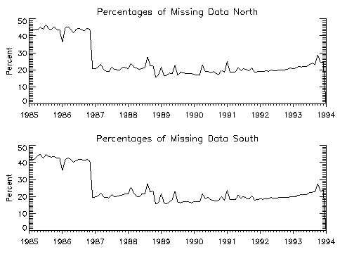
The amount of missing data in the ISCCP data set is large. For
1985-1986 on average, 45% of ISCCP data are missing. For 1987-1993
this figure is lower, roughly 20%. This drop in percentage
of missing data most likely correlates with a change in the satellite reporting
the data. In the ISCCP data set, a missing data cell retains the
cell indices and the TOVS atmospheric information. The remaining
data for the cell is set to a nodata value of 255.
The easiest way to fill the missing data is with daily average values. In the interest of time, this is the course that was chosen but, this may be revisited in the future.
For daytime, ISCCP reports values for variables derived from both visible and IR measurements. For nighttime, in the absence of sunlight, only the IR derived variables are reported. According to the ISCCP documentation, the VIS/IR retrieval is superior to the IR only retrieval. When VIS data is available ISCCP reports more detailed cloud information compared with the IR only case. The way the processing code is currently written, either the VIS data are used for cloud properties or the IR data are used but, not both. Prfv2.pro, the current version of the prf code, uses the VIS data when available (i.e. during the day) and the IR when VIS is not available (i.e. at night). When considering how to calculate the daily average cloud properties a decision had to be made whether to use VIS or IR data. VIS data would provide more detailed cloud information but IR data could potentially be available for more times throughout the 24 hour period. The issue was whether to have fewer but more detailed data points to average or less detailed but more frequent data points to average. A compromise was reached whereby, if VIS data is reported for at least half the day ( minimum of 4 out of the 8 3-hourly time steps) the VIS data is used to calculate daily average cloud properties. If there is less than half a day of VIS data then the majority data type reported for the day, VIS or IR, is used for calculating daily averages. For variables other than cloud properties all available data are used to calculated the daily average.
For missing data the following filling techniques are used for the variables required by fluxnet:
There are some days with grid cells for which no data is reported for
the entire day. No attempt was made to fill these cells. In
the daily average product, these cells have a nodata value of -999.
Such days and cells where not included in calculating the monthly average
product. For a list of days and cells with no data reported for the
entire day please click here.
The above procedure outlines the assumptions necessary to create an input case data set for the neural net implementation of Streamer (Fluxnet). This IDL code is in the file prfv2.pro. Very similar code is used to generate the input training data for the neural net (trainG.pro).
The main limitations arise from the information content and quality of the ISCCP and PathP data sets. For example, our calculated surface type information is a crude approximation devised to maintain the reported albedo, but lacking much hard data on what is actually there. Any improved knowledge of surface type would increase the validity of the flux data. The temperature and water vapor profiles are also of concern, as the temperature profile fixes the position of clouds, and the water vapor affects directly the longwave fluxes. The code contains a variety of measures to ensure the integrity of these profiles. The largest errors most likely occur as a result of having to use profiles from adjacent cells when the profile in the current cell contains significant errors. In general, the water vapor profiles are more trouble than the temperature - with more unreported values and missing profiles. The PathP data seems to be of much higher quality when it is reported, and so it is preferred, but there is the concern about the relevance of such a profile, collected for a much smaller cell perhaps located some distance away, to the cloud amounts of a larger cell.
The data filling technique used to compensate for missing data is very simple. There are probably more involved methods that would provide better estimates. Such alternatives may be explored in the future, as time permits.
Both data sets throw out the occasional unphysical value for some parameter or another. All the parameters are not rigorously screened for bad values; rather, with all the experience with running the various bits of code, I have added code to deal with any spurious values that have previously appeared. HOWEVER, with more years of data becoming available, with, potentially, different spurious value problems, THE CODE MIGHT CRASH!!
If the ISCCP data is reprocessed at some point to fix errors or improve
accuracy, the neural net should be retrained.