| FTP Site | Validation Info | Problems | Credits |
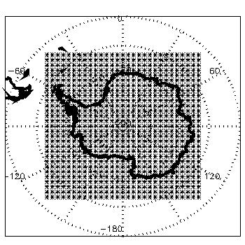
Data from the extended Advanced Very High Resolution Radiometer (APP-x) data set were used to force the Arctic Regional Climate System Model (ARCSyM) (Lynch et al., 1995; Baily and Lynch, 2000a; Baily and Lynch, 2000b). Click here for information concerning the APP-x data set. ARCSyM has as its heritage the National Center for Atmospheric Research (NCAR) Regional Climate Model Version 2 (Giorgi et al., 1993a and Giorgi et al., 1993b), which utilizes a hydrostatic primitive equation atmospheric model. The ARCSyM, however, is specifically designed to simulate the coupled ocean-ice-atmosphere system in the polar regions. The ARCSyM staggered "Arakawa B" (Arakawa and Lamb, 1977) horizontal grid was set to a resolution of 200 km for all model simulations, chosen for computational efficiency. Click here to see the ARCSyM horizontal domain. In addition, 23 terrain-following vertical sigma levels, with the greatest resolution in the boundary layer, were used for all model simulations. The lowest sigma level used is 0.99, which is about 40 m above the ground. The pressure at the model top was set to 50 mb. The model was initialized and forced at the lateral boundaries with European Center for Medium-Range Weather Forecasts (ECMWF) analyses (Trenberth, 1992) using a sponge boundary condition at 00Z and 12Z.
The NCAR Community Climate Model 2 (CCM2) shortwave radiation scheme (Briegleb, 1992), the Rapid Radiative Transfer Model (RRTM, Mlawer et al., 1997) longwave radiation model, the planetary boundary layer scheme of Holtslag et al. (1990), and the NCAR Land Surface Model (LSM, Bonan, 1996) were employed for all simulations. An implicit moisture scheme (Giorgi et al., 1993a) was used because Hines et al. (1997) showed that the more comprehensive explicit moisture scheme of Hsie et al. (1984) did not perform well in the Antarctic. Convective processes were not included. This should have a minimal impact on the results because significant convection occurs relatively infrequently in the Antarctic, especially over the Antarctic continent. The thermodynamic sea ice model of Parkinson and Washington (1979) with modification by Schramm et al. (1997) was used. A dynamic sea ice model was not utilized because sea ice concentration was initialized and updated every day at 00Z from the 25 km Scanning Multichannel Microwave Radiometer (SMMR) sea ice concentration product prior to about July 1987, and from the Special Sensor Microwave/Imager (SSM/I) sea ice concentration product (Comiso, 1999) thereafter.
Water vapor amounts in the ARCSyM are adjusted during the model simulations such that the horizontal and vertical location of clouds in the model more closely match satellite observations, under the assumption that the satellite-derived clouds are more realistic than the modeled cloud fields. The resolution of the APP-x data set was first converted from 25 km to 200 km to match the ARCSyM grid. This was accomplished by averaging the cloud optical depth, cloud particle size, and cloud top pressure from the APP-x data set in a given ARCSyM grid cell, where the grid cell boundaries are defined by the dot points on the "Arakawa B" horizontal grid. Cloud thermodynamic phase and cloud amount require a different treatment, where the 200 km resolution cloud phase was taken to be the mode of the 25 km phase retrievals (either water or ice) that fall within each ARCSyM grid cell, and the cloud fraction was the number of cloudy APP-x pixels divided by the total number of pixels within each ARCSyM grid cell. The geometric cloud thickness for each 200 km grid cell was calculated as the cloud visible optical depth multiplied by the extinction coefficient, which is based on the cloud particle size and phase. If all of the 25 km APP-x values within a given grid cell were missing then the grid cell value was also missing. This rarely occurred. Surface temperature from the APP-x data set was also spatially smoothed onto the ARCSyM grid, and any missing grid cell values were filled using a kringing procedure. If an entire day of surface temperature data was missing, then linear interpolation is used to fill in the missing day. The APP-x surface temperatures were used to initialize and update the ARCSyM sea surface temperatures (SST's) at 00Z in model time. Sea ice concentrations were obtained from the SSMR and SSM/I 25 km sea ice concentration data sets provided by the National Snow and Ice Data Center. The 200 km resolution values were determined in the same manner as the SST's. The sea ice concentration data is initialized and updated in the model at the same time as the SST's.
The cloud fraction in each grid cell determined the horizontal locations where water vapor is to be added and subtracted. If the cloud fraction for a specific grid cell was 50% or greater, then that grid cell was taken to be cloudy, otherwise it was considered clear. Determining the location of a given cloud in the vertical is not quite as straightforward. The cloud top pressure from the APP-x data set was converted to a cloud top sigma level using 50 mb as the pressure value at the top of each column and the surface pressure for a given grid cell from the ECMWF analysis. The calculated cloud top sigma level is then matched to the closest model sigma level and the geopotential height at the cloud top is taken to be the geopotential height of the ECMWF analysis at that sigma level. The cloud base is then determined by subtracting the geometric cloud thickness based on the APP-x cloud properties from the geopotential height at the cloud top. The geopotential height in the ECMWF analysis that most closely matches the calculated geopotential height at the cloud base is found and the sigma value at that model level is taken to be the cloud base sigma level. The base of any cloud that was found to extend below the surface was reset to the 0.99 sigma level. All sigma levels including and between the cloud base and the cloud top were flagged so that at the appropriate model time water vapor would be added to those levels, if a cloud is not already present in the model. Next, all grid cells that were determined to be "clear" based on the satellite data were checked for the presence of clouds. If a cloud was present in the model, then water vapor was subtracted.
ECMWF analyses interpolated to the ARCSyM grid were obtained for 00Z and 12Z for the time frame of interest. The ECMWF data was then linearly interpolated in time so that boundary forcing data was available every three hours beginning at 00Z and ending at 21Z. The water vapor fields within the regions of the domain that were within 1.5 hours of either APP-x composite time were updated along with the domain boundaries every 3 hours. In order to force the model with the APP-x data, water vapor was simply added or subtracted at the appropriate sigma levels where clouds or clear sky were indicated in the APP-x data. Using an implicit moisture scheme, enough water vapor was added to make the air slightly supersaturated (relative humidity (RH) = 101%) if a cloud was indicated by the APP-x data. If clear sky was indicated by the satellite data, water vapor was subtracted so that the air was sufficiently below saturation (RH = 80%). The latent heat release associated with forcing net condensation or net evaporation in the model should have little impact on the results. This is especially true in dry Antarctic atmosphere. All model integrations were 48 hours. A model "spin-up" was allowed for by discarding the first 24 hours of output and keeping only the second 24 hours of output. Daily means were then computed from 00Z, 06Z, 12Z, and 18Z model output. Monthly means were computed from the daily means. Surface fluxes for one year of the data set (1987) have been validated against surface measurements at the South Pole and over the Ross Ice Shelf. Click here for validation information.
Monthly averages of the parameters listed in Table 1 below are available for 1987 - 1997 in HDF. The naming convention is as follows: yymm.monthly.hdf, where yy is the two digit year and mm is the two digit month. All parameters with the exception of the zonal and meridional wind vectors are defined on the cross points of the "Arakawa B" grid. The wind vectors are defined on the dot points of the grid. All radiative fluxes are taken to be positive and the turbulent fluxes are positive when directed towards the surface. In addition, all parameters are stored as 32-bit floating point numbers. IDL software is provided to read in data from the HDF parameter files and the file constantfields.input.hdf which contains latitude and longitude at the cross points and dot points along with the other parameters listed in Table 2 below. Click here to access the data and IDL software.
No data is available from October 1994 through December 1994 due to the lack of AVHRR data during this period.
Arakawa, A., and V.R. Lamb, 1977: Computational design of the basic dynamical process of the UCLA general circulation model. Methods in Comp. Physics, 17, Academic Press, 173-265.
Baily, D.A. and A.H. Lynch, 2000a: Development of an Antarctic regional climate system model. Part I: Sea ice and large scale circulation. J. Climate, 13, 1337-1350.
Baily, D.A. and A.H. Lynch, 2000b: Development of an Antarctic regional climate system mode. Part II: Station validation and surface energy balance. J. Climate, 13, 1351-1361.
Bonan, G.B., 1996: A land surface model (LSM Version 1.0) for ecological, hydrological, and atmospheric studies: Technical description and user's guide. NCAR Tech. Note NCAR/TN-417_STR, 150 pp.
Briegleb, B.P., 1992: Delta Eddington approximation for solar radiation in the NCAR Community Climate Model. J. Geophys. Res., 97, 7603-7612.
Comiso, J., 2002: Bootstrap sea ice concentrations from Nimbus-7 SMMR and DMSP SSM/I. Boulder, CO, USA: National Snow and Ice Data Center. Digital Media.
Giorgi, F., M.R. Marinucci, and G.T. Bates, 1993a: Development of a Second Generation Regional Climate Model (RegCM2). Part I: Boundary-layer and radiative transfer processes. Mon. Wea. Rev., 121, 2794-2812.
Giorgi, F., M.R. Marinucci, and G.T. Bates, 1993b: Development of a Second Generation Regional Climate Model (RegCM2). Part II: Convective processes and assimilation of lateral boundary conditions. Mon. Wea. Rev., 121, 2814-2832
Hines, K.M., D.H. Bromwich, and R.I. Cullather, 1997: Evaluating moist physics for Antarctic mesoscale simulations, Ann. Glaciol., 25, 282-286.
Holtslag, A.A.M., E.I.F. Debruijn, and H.L. Pan, 1990: A high resolution air-mass transformation model for short-range weather forecasting. Mon. Wea. Rev., 118 (8), 1561-1575.
Hsie, E.Y., R.A. Anthes, and D. Keyser, 1984: Numerical simulation of frontogenesis in a moist atmosphere. J. Atmos. Sci., 41, 2581-2594.
Lynch, A.H., W.L. Chapman, J.E. Walsh, and G. Weller, 1995: Development of a regional climate model of the Western Arctic. J. Climate, 8, 1555-1570.
Mlawer, E.J., S.J. Taubman, P.D. Brown, M.J. Iacono, and S.A. Clough, 1997: Radiative transfer for inhomogeneous atmospheres: RRTM, a validated correlated-K model for the longwave. Geophys. Res., 102 (D14), 16663-16682.
Parkinson, C.L. and W.M. Washington, 1979: A large-scale numerical model of sea-ice. J. Geophys. Res., 84, 311-337.
Schramm, J.L., M. Holland, J.A. Curry, and E.E. Ebert, 1997: Modeling the thermodynamics of a distribution of sea ice thickness. Part I: Sensitivity to ice thickness resolution. J. Geophys. Res., 102, 23079-23092.
Trenberth, K.E., 1992: Global analyses from ECMWF and atlas of 1000 to 10 mb circulation statistics. NCAR Tech. Note TN-373+STR, 191 pp.